Forum Members,
I'm new to numbers and would like some assistance in using conditional formatting.
What I have done:
Looked at various you tube videos and read forums in order to find help.
Problem:
I'm building a sheet to track due dates.
1. need to track 45 day mark, 60 and 90 day mark, from initial notification
- First cell to the following (G16+45), this will give me a date which is 45 days in the future form the initial notification date.
- second cell is set to (G16+60), this will give me a date which is 60 days in the future from the initial notification date.
- Third cell is set to (G16+90), this will give me a date which is 90 days in the future from the initial notification date.
-if the initial notification date is 15 July 2017, numbers give me a 45 day of 29 Aug 2017; a 60 day of 13 Sept 2017; and a 90 day of 13 Oct 2017.
Show date: is the date an individual shows up
2. Conditional Formating (need help with)
1. If current date is equal to or greater than 45 day mark then strike out and fill blue
2. If current date is equal to or greater than 60 day mark then strike out and fill orange
3. If current date is equal to or greater than 90 day mark then strike out and fill red
if show date is less than 45 day mark then stop rules 1-3 as stated above
if who date is less than 60 day mark then stop rule for 90 day mark (3) but still strike out 45 day mark
if show date is less than 90 day mark then stop rule (3) but still continue with rule 1 and 2
if show is not inputed on the 90 day mark then apply rules 1 through 3 and input "stop" on cell containing show date
thanks in advance
77XX
I'm new to numbers and would like some assistance in using conditional formatting.
What I have done:
Looked at various you tube videos and read forums in order to find help.
Problem:
I'm building a sheet to track due dates.
1. need to track 45 day mark, 60 and 90 day mark, from initial notification
- First cell to the following (G16+45), this will give me a date which is 45 days in the future form the initial notification date.
- second cell is set to (G16+60), this will give me a date which is 60 days in the future from the initial notification date.
- Third cell is set to (G16+90), this will give me a date which is 90 days in the future from the initial notification date.
-if the initial notification date is 15 July 2017, numbers give me a 45 day of 29 Aug 2017; a 60 day of 13 Sept 2017; and a 90 day of 13 Oct 2017.
Show date: is the date an individual shows up
2. Conditional Formating (need help with)
1. If current date is equal to or greater than 45 day mark then strike out and fill blue
2. If current date is equal to or greater than 60 day mark then strike out and fill orange
3. If current date is equal to or greater than 90 day mark then strike out and fill red
if show date is less than 45 day mark then stop rules 1-3 as stated above
if who date is less than 60 day mark then stop rule for 90 day mark (3) but still strike out 45 day mark
if show date is less than 90 day mark then stop rule (3) but still continue with rule 1 and 2
if show is not inputed on the 90 day mark then apply rules 1 through 3 and input "stop" on cell containing show date
thanks in advance
77XX